Del estudio observacional y el ajuste a la decisión clínica. Parte 2
Rev Argent Cardiol 2024;92:379-385. http://dx.doi.org/10.7775/rac.v92.i5.20823
Correspondence: Arturo Cagide. E-mail: arturo.cagide@hospitalitaliano.org.ar
MTSAC Miembro Titular de la Sociedad Argentina de Cardiología
2024 ©Revista Argentina de Cardiología

In this second part, we continue to explain the statistical methods, from the most common to the most novel, for the analysis of observational studies.
Propensity Score (PS)
The goal of this methodology is to adjust for confounders so that they are balanced between the intervention and control groups.
Figure 1 illustrates the procedure. The first step is to estimate the statistical association between confounders (or independent variables) and exposure (or dependent variable), again using multivariate analysis (logistic regression).
Fig. 1
Propensity score (PS) and derived analysis 40.
The final objective of the study is, as in Fig. 4 (Part 1), to estimate the possible association of the exposure with the outcome. Previously, the association of confounders with exposure is analyzed and the PS is calculated. Then, the PS enables the estimation of the independent association between the exposure and the outcome through the application of diverse statistical methodologies.
IPTW: inverse probability of treatment weighting; LR: logistic regression
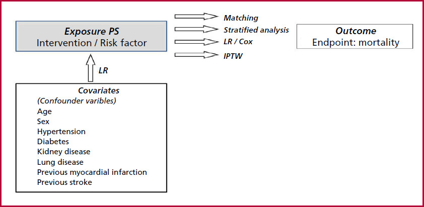
The propensity score (PS), which represents the likelihood of being exposed to the intervention, adjusted for the presence of confounding factors, is derived from the resulting data.
One benefit of PS over multivariate analysis is that the number of independent variables is not constrained by the prevalence of the treatment. This is because the treatment, intervention, or prognostic factor, in contrast to the outcome, will consistently have a sufficient number of observations. (1)
There is some debate regarding the variables that should be included in the calculation of the PS. In general, all the variables that the investigator deems relevant to a given treatment or intervention should be included. Basically, the variables determining the outcome should also be included. (2),(3)
As is the case with any multivariate analysis, the issue is that only known and available independent variables are taken into account. Consequently, the PS may be flawed in predicting exposure to treatment or intervention as a result of that situation.
The ROC curve can be used to evaluate the model in the calculation of the PS. While there is some disagreement about the exact value that should be considered adequate, most authors place it in an area under the curve of 0.80.
There are several procedures to evaluate the association of the intervention with the endpoint (Figure 1). (4)
a) Matching
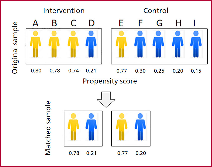
In accordance with the aforementioned methodology, each individual will be characterized according to their baseline characteristics or confounding factors, as determined by a specific PS. Some individuals in the intervention group will have a PS similar to those in the control group, so that it is possible to match patients from both groups according to their PS. (Figure 2)
Fig. 2
Matching 58.
Theoretical example of a study of 220 patients, 120 in the intervention group and 100 in the control group. The PS for the entire sample (center), the intervention group (top), and the control group (bottom) is plotted on a scale of increasing values. Each subject in the intervention group is matched with a subject in the control group with an equal or very close PS. This process results in 18 pairs, reducing the original sample size to 16%. (36/220). In the matched sample, confounders from both the intervention group and the control group are "balanced".

This process generates a (matched) subpopulation whose confounders are balanced between both groups in such a way that they no longer influence on the estimation of the association of the intervention with the outcome.
However, a significant number of individuals from both treated and untreated groups will be excluded because the corresponding pair is not available. This number of excluded individuals is directly related to the level of confounder imbalance between both groups in the original study sample.
Thus, the conclusion of the study and its translation into practice is limited exclusively to the matched sample and cannot be extrapolated to the entire population.
b) Multivariate analysis and PS
An analysis of this type can be performed by including the intervention (or the prognostic criterion according to the case) and the PS, which represents all the confounders analyzed, as independent variables.
c) Stratified analysis
This method, like multivariate analysis, includes all individuals in the trial. The procedure entails forming strata in accordance with the PS and estimating the association between the exposure variable and the outcome in each stratum. This is followed by the calculation of an overall result, which represents this association (Figure 3).
Fig. 3
Stratified analysis 75.
The individuals were grouped into quintiles according to their PS. The relative risk (RR) for the outcome (e.g., mortality) was estimated for each quintile. The RR of the sample adjusted for the PS and the confounding variables included in it is then calculated.

The standard stratified analysis for confounder balance presents a challenge when attempting to adjust for only some variables. This is because the number of strata increases exponentially when incorporating numerous criteria with few observations in each of them. Applying stratification according to PS incorporates all the baseline characteristics of interest, as confounders.
d) Inverse probability of treatment weighting (IPTW)
Unlike matching, but similar to stratified analysis, this method includes the entire sample under study.
However, while matching achieves adjustment by reducing the population until the confounders are matched in the groups to be compared, with IPTW this objective is achieved by increasing the population with individuals with a similar rate of confounders using a mathematical technique. (5)
Figure 4 is a theoretical example comparing an intervention group with a control group. Age, dichotomized into < 50 and ≥ 50 years, is for this example, the only confounder. In the intervention group there are four subjects, 3 < 50 years and 1 ≥ 50 years; in the control group there are 5 subjects, 1 < 50 years and 4 ≥ 50 years.
Fig. 4
Matching 88. 89.
Theoretical example of a study comparing an intervention group of 4 individuals with a control group of 5 individuals. The PS was calculated in each group. Age is the confounding variable: <50 years in yellow and ≥50 years in blue. To adjust for age, individuals from each group are matched with those with similar PS values. The original sample of 9 individuals is reduced to 2 pairs (4 individuals).
The age-adjusted sample has been significantly reduced in number.
The age must be adjusted so that both groups can be compared in terms of a given outcome, for example mortality. For this purpose, the PS, as previously mentioned, is estimated for each group which will undoubtedly be different for each individual.
If the matching strategy were applied, two pairs of 2 patients each, treated and control, could be integrated (Figure 4) sharing similar PS, so that the sample would be limited to only 4 individuals.
Let us now examine the example illustrated in Figure 5.
Fig. 5
Inverse probability of treatment weighting (IPTW) 97.
The upper part shows the condition of Fig. 4. The aim is to adjust for age (which in this theoretical example is the only existing confounder), dichotomized into < 50 years (in yellow) and ≥ 50 years (in blue). In individuals < 50 years the probability of receiving the intervention, which is the same in all of them, is 3/4 = 0.75. In those ≥ 50 years the probability of receiving the intervention, which is also the same in all of them, is 1/5 = 0.20. The probabilities calculated in this theoretical case, arising from a simple mathematical calculation, constitute the PS. (The probability of receiving control treatment will be 1 - PS).
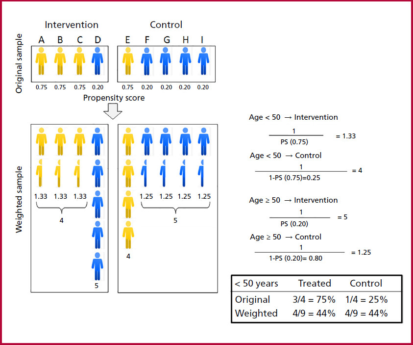
In contrast to Fig. 4, let us now assume that there is again only one confounder, age.
The probability of receiving the intervention (the PS) in individuals < 50 years is 0.75, while the probability in those ≥ 50 years is 0.20.
Note that with the same probability of receiving the intervention (PS = 0.75), 3 individuals < 50 years received it and only 1 did not (in the control group). In turn, in those ≥ 50 years with the same probability of receiving the intervention (PS = 0.20) or being in the control group (1-PS = 1-0.20 = 0.80) 4 did not receive the intervention and only 1 received it.
Applying IPTW:
-
< 50 years: the inverse probability of receiving treatment is 1.33 (1/0.75). Each individual < 50 years who received the intervention will now be represented by 1.33, so that the sum of all of them is 4. The inverse probability of not receiving treatment is 4 [1/1-0.75; the probability of not receiving the intervention is 1 minus the probability of intervention, (1-PS)]: the only subject < 50 years in the control group will be represented by 4 (Figure 5).
-
≥ 50 years: the inverse probability of receiving the intervention is 5 (1/0.20): in the intervention group the only individual ≥ 50 years will be represented by 5. The inverse probability of being in the control group is 1.25 (1/1-0.20): each individual in the control group ≥ 50 years will be represented by 1.25, so that the sum of all of them is 5.
The formulas illustrate the methodology for calculating the IPTW, which allows for the estimation of how each individual will be represented in the intervention and control groups. The table shows the distribution by age before and after adjustment, which in this particular case is perfect. See explanation in the text.
Please note that in the original sample, the ratio of individuals < 50 years with and without treatment was 3:1. Once IPTW has been applied, the sample is fully balanced in 4. In turn, in ≥ 50 years with and without treatment the original ratio of 1:4 remained equalized at 5.
Thus, the IPTW method achieves pseudo-randomization by generating a pseudo-population in which the adjustment for the variable age is mathematically perfect (Figure 5).
The situation described is particularly relevant when considering only one confounding factor. Before adjustment, the PS was the same across all individuals < 50 years (0.75), and those ≥ 50 also exhibited the same PS (0.20).
In a real-world setting, the probability of treatment is influenced by a number of confounding factors. The global effect of these confounders is represented in the PS which will vary from case to case (Figure 6).
The adjustment using IPTW is similar to that explained in Figure 5, applying the individual PS of each patient. The adjustment reduces the imbalance, although certain differences in age distribution between the groups with and without treatment persist due to the fact that other confounders, besides age, influence on the PS. (6)
Fig. 6
Inverse probability of treatment weighting (IPTW) 121.
Unlike the previous example, the probabilities calculated by the PS vary from one individual to another, as they are influenced not only by age but also by the entire range of confounding variables. Their estimation results from a logistic regression analysis of the covariates with the treatment received (intervention or control). The application of the same methodology illustrated in Figure 5 results in a reduction of the differences, although the adjustment is not mathematically exact. See explanation in the text.

The strategy described for the variable age should be applied to all the variables or confounders available considered in the calculation of PS.
Estimating the level of adjustment
It is of the utmost importance to ensure the precision of the adjustment when applying the IPTW, as it encompasses the entire population under study, which is likely to exhibit significant differences in the prevalence of multiple confounders. In the case of matching, there may also be imbalance, although to a lesser extent.
To evaluate the level of adjustment achieved, the absolute standardized difference (ASD) is usually used, which is the difference measured in units of the standard deviation for each of the confounding variables after adjustment using IPTW. In general, a difference < 0.10 is deemed an acceptable margin that ensures the adjustment was adequate. However, in some cases, this extends to 0.20, which may detract from the consistency of the conclusions of the study.
Sometimes the ASD is plotted before and after the adjustment to indicate the previous imbalance and the success of the adjustment.
The accuracy of the PS for estimating the probability of being intervened is a conditioning factor of the IPTW methodology. Again, the confounding variables not included, whether unknown or not contemplated, constitute a critical aspect of the statistical procedure.
Back into clinical trials from a methodological perspective
We invite readers to revisit Part 1 of this review to gain a comprehensive understanding of the following considerations.
Trial 1 (7)
-
After adjusting for confounders using PS matching, the analysis was conducted on a subset of 1866 patients from the original sample of 9586: 933 in the percutaneous coronary intervention (PCI) group and 933 in the medical treatment (MT) group, that is, 933 pairs. It is evident that there was a significant imbalance regarding certain baseline characteristics. Consequently, PCI was only performed on a selected group of patients with a favorable prognosis. It is therefore essential to address these discrepancies to ensure the validity of the results.
-
Such correction was adequate since the standardized difference was < 0.05 for most of the 20 variables considered.
-
The adjusted HR of the outcome mortality/nonfatal myocardial infarction (1.49, MT versus PCI) was calculated in the matched sample according to the multivariate Cox model. This was done with the intention of adjusting for any remaining differences by incorporating certain variables.
-
The translation of this trial into clinical practice is limited exclusively to the matched group of patients, 85% of the MT group, but only 11% of those in the PCI group.
Trial 2 (8)
-
In this case the adjustment was made using IPTW.
-
The standardized difference was < 0.05 for all the 13 variables considered (Table 2, Part 1).
-
In addition to the standardized difference, Figure 2 illustrates the effect on the outcome with a relative risk of 0.72. This indicates that patients with prior statin use had a 28% reduction in heart failure as a complication of acute coronary syndrome.
Trial 3 (9)
-
The effect of the intervention was estimated using PS according to three statistical criteria (Table 3, Part 1). 152.
-
IPTW (primary analysis): no benefit of anticoagulation in CHADS2 patients ≤ 1, but there was difference in the incidence of major bleeding, which was significantly more common in the treated group.
-
matching and Cox model (secondary and sensitivity analysis). The result showed no benefit of anticoagulation with higher bleeding rate in CHADS2 ≤ 1. This finding aligns with the post-IPTW analysis.
-
-
It is interesting to analyze Figure 1 (Part 1) beyond the result in patients with CHADS2 ≤ 1, which illustrates the standardized difference before and after adjustment. The limit of 0.1 defines the criterion for the level of adjustment. The difference before adjustment was significantly greater in individuals with a CHADS2 score ≤ 1 compared to those with a score of 2. This demonstrates that the variables probably associated with thromboembolism in the former group were markedly different in patients without anticoagulation (low prevalence) compared to those who did not receive such treatment (high prevalence).
Trial 4 (10)
-
This is a prognostic study on the risk of type 2 versus type 1 myocardial infarction using IPTW.
-
The standardized difference is illustrated in a chart similar to that in Figure 1 (Part 1), but it is clear that the two charts are different. Firstly, the acceptance limit is set at a value < 0.2, which is twice as high as in the previous case. Furthermore, following the adjustment, the differences remained significant, at approximately 0.10. It is possible that the sample size used in relation to the number of covariates was incorrect, resulting in the incorrect calculation of PS.
-
The conclusion of the study is limited by imperfect adjustment for confounders (comorbidities).
Trial 5 (11)
-
In this case, the aim of this trial was not to evaluate the effect of an intervention or the prognostic value of a new criterion, but to determine the outcome of aortic stenosis. The problem is that in one group of patients, the intervention effectively interrupted the natural history, potentially introducing bias in the non-intervened group (higher risk due to having individuals at lower risk for the intervention) or, conversely, having selected those at high risk for the procedure.
-
The IPTW was not designed to compare the treated group with the untreated group. Rather, it was intended to adjust both populations and then compare the adjusted results with the original, untreated population. Table 4 (Part 1) does not detail the standardized difference but compares mortality of the adjusted sample with that of the unadjusted sample in subgroups according to the severity of valvular heart disease.
-
For the authors, the non-interventional group represents the actual natural history of aortic stenosis unaffected by the intervention.
Conclusion
Randomized studies undoubtedly constitute the highest level of evidence. However, they are also the most complex, time-consuming, and costly studies. Only a few interventions can be evaluated by this methodology.
Observational trials represent a viable option for the evaluation of new prognostic criteria or innovative therapeutic alternatives, particularly when large prospective databases are available. In this context, statistical methodology presents a significant challenge in terms of correcting for variables that may affect the association being studied.
It is crucial for clinicians to become familiar with the terminology, tables, and charts associated with the statistical strategy employed to assess the effect, as this knowledge is vital for decision-making. It is not a matter of understanding the mathematical complexities involved, but rather the conceptual basis.
Failure to learn these concepts will result in an unquestioning acceptance of expert opinions. It is always preferable to analyze the basic information rather than to resort to that interpreted by others.
Ethical considerations
Not applicable.
Conflicts of interest
None declared.(See authors conflicts of interest forms in the website).
REFERENCES
1. Andrew BY, Alan Brookhart M, Pearse R, Raghunathan K, Krishnamoorthy V. Propensity score methods in observational research: brief review and guide for authors. Br J Anaesth 2023 131:805-9. https://doi.org/10.1016/j.bja.2023.06.054 .
2. Deb S, Austin PC, Tu JV, Ko DT, Mazer CD, Kiss A, Fremes SE. A Review of Propensity-Score Methods and Their Use in Cardiovascular Research. Can J Cardiol 2016;32:259-65. https://doi.org/10.1016/j.cjca.2015.05.015 .
3. Benedetto U, Head SJ, Angelini GD, Blackstone EH. Statistical primer: propensity score matching and its alternatives. Eur J Cardiothorac Surg 2018;53:1112-7. https://doi.org/10.1093/ejcts/ezy167 .
4. Johnson SR, Tomlinson GA, Hawker GA, Granton JT, Feldman BM. Propensity Score Methods for Bias Reduction in Observational Studies of Treatment Effect. Rheum Dis Clin North Am 2018;44:203-13. https://doi.org/10.1016/j.rdc.2018.01.002.
5. Austin PC, Stuart EA. Moving towards best practice when using inverse probability of treatment weighting (IPTW) using the propensity score to estimate causal treatment effects in observational studies. Stat Med 2015;34:3661-79. https://doi.org/10.1002/sim.6607 .
6. Chesnaye NC, Stel VS, Tripepi G, Dekker FW, Fu EL, Zoccali C, et al An introduction to inverse probability of treatment weighting in observational research. Clin Kidney J 2021;15:14-20. https://doi.org/10.1093/ckj/sfab158 .
7. Hannan EL, Samadashvili Z, Cozzens K, Walford G, Jacobs AK, Holmes DR Jr, et al. Comparative outcomes for patients who do and do not undergo percutaneous coronary intervention for stable coronary artery disease in New York. Circulation 2012;125:1870-9.https://doi.org/10.1161/CIRCULATIONAHA.111.071811
8. Bugiardini R, Yoon J, Mendieta G, Kedev S, Zdravkovic M, Vasiljevic Z, et al. Reduced Heart Failure and Mortality in Patients Receiving Statin Therapy Before Initial Acute Coronary Syndrome. J Am Coll Cardiol 2022;79:2021-33.https://doi.org/10.1016/j.jacc.2022.03.354
9. Kanaoka K, Nishida T, Iwanaga Y, Nakai M, Tonegawa-Kuji R, Nishioka Y, et al. Oral anticoagulation after atrial fibrillation catheter ablation: benefits and risks. Eur Heart J. 2024;45:522-34.https://doi.org/10.1093/eurheartj/ehad798
11. Généreux P, Sharma RP, Cubeddu RJ, Aaron L, Abdelfattah OM, Koulogiannis KP, et al. The Mortality Burden of Untreated Aortic Stenosis. J Am Coll Cardiol 2023;82:2101-9. https://doi.org/10.1016/j.jacc.2023.09.796